Tuan Anh Le
Occam’s Razor and Model Selection
21 February 2017
Given different models \(\mathcal M_k, k = 1, \dotsc, K\) of data \(y\), how can we make predictions?
Inference
If we assume that \(\mathcal M_k\) is the correct model, we can perform posterior inference on latent variables \(x\): \begin{align} p(x \given y, \mathcal M_k) &= \frac{p(y \given x, \mathcal M_k)p(x \given \mathcal M_k)}{p(y \given \mathcal M_k)} \end{align} where
- \(p(x \given \mathcal M_k)\) is the prior,
- \(p(y \given x, \mathcal M_k)\) is the likelihood,
- \(p(y \given \mathcal M_k) = \int_{\mathcal X} p(y \given x, \mathcal M_k)p(x \given \mathcal M_k) \,\mathrm dx\) is the evidence.
Bayesian Model Averaging
Let’s go one level higher and perform inference on the models: \begin{align} p(\mathcal M_k \given y) = \frac{p(y \given \mathcal M_k) p(\mathcal M_k)}{p(y)} \end{align} where
- \(p(\mathcal M_k)\) is the prior over models,
- \(p(y \given \mathcal M_k)\) is the evidence (from before),
- \(p(y)\) is the normalizing constant.
We would like to actually know \(p(x \given y)\) and its expectations with respect to various functions.
To calculate this, we do the following (which is usually called Bayesian model averaging):
\begin{align}
p(x \given y) &= \sum_{k = 1}^K p(x, \mathcal M_k \given y) \
&= \sum_{k = 1}^K p(x \given y, \mathcal M_k) p(\mathcal M_k \given y)
\end{align}
where
- \(p(x \given y, \mathcal M_k)\) is the posterior given the model \(\mathcal M_k\) and
- \(p(\mathcal M_k \given y)\) is the model posterior.
This is what we would like to do ideally but it can be very difficult, in which case we turn to a poor man’s Bayesian model averaging – Bayesian model selection. Think of finding the maximum a-posteriori estimate instead of doing posterior inference.
Bayesian Model Selection
Here, we assume that we can’t do Bayesian model averaging and turn into Bayesian model selection. We want to find the best model: \begin{align} \mathcal M^\ast = \argmax_{\mathcal M_k} p(\mathcal M_k \given y) \end{align}
We see that to compare two models \(\mathcal M_i\) and \(\mathcal M_j\), we just need to compare
- \(p(y \given \mathcal M_i) p(\mathcal M_i)\) and
- \(p(y \given \mathcal M_j) p(\mathcal M_j)\).
The prior over models is usually uniform (we don’t prefer any model a priori). Hence, we can compare the evidence to select the best model.
Occam’s Razor
The principle of Occam’s razor says that we should prefer simple models over complicated ones. Bayesian model selection has a somewhat built-in Occam’s razor. A model \(\mathcal M_k\) is complex if the probability mass of \(p(y \given \mathcal M_k)\) is spread around a large area of \(y\). Because a probability distribution must integrate to one, a model being more complex means that it assigns a lower value of \(p(y \given \mathcal M_k)\) to data. On the other hand, if the model is too simple, it won’t assign any probability to \(y\) that is not modeled. We must somehow pick a model that is just right. See illustration below.
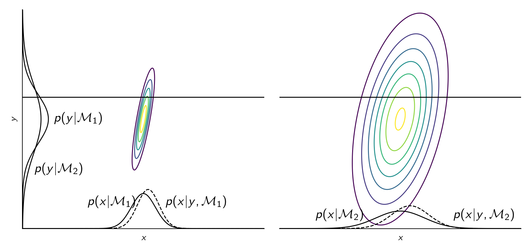 Jupyter notebook for generating this plot
Note that a model having a lot of parameters doesn’t mean that it is complex. It’s only complex if \(p(y \given \mathcal M_k)\) is spread around a large area of \(y\).
References
- Rasmussen, C. E., & Ghahramani, Z. (2001). Occam’s razor. Advances in Neural Information Processing Systems, 294–300.
@article{rasmussen2001occam, title = {Occam's razor}, author = {Rasmussen, Carl Edward and Ghahramani, Zoubin}, journal = {Advances in neural information processing systems}, pages = {294--300}, year = {2001}, publisher = {MIT; 1998} } - Ghahramani, Z., & Murray, I. (2005). A note on the evidence and Bayesian Occam’s razor. Gatsby Unit Technical Report GCNU-TR 2005–003.
@techreport{ghahramani2005note, title = {A note on the evidence and Bayesian Occam's razor}, author = {Ghahramani, Zoubin and Murray, Iain}, year = {2005}, institution = {Gatsby Unit Technical Report GCNU-TR 2005--003} } - MacKay, D. J. C. (2003). Information theory, inference and learning algorithms. Cambridge university press.
@book{mackay2003information,
  title = {Information theory, inference and learning algorithms},
  author = {MacKay, David JC},
  year = {2003},
  publisher = {Cambridge university press}
}
[back]