Tuan Anh Le
Learning and amortized inference in hierarchical Bayesian models
04 September 2020
Say you hear people speaking in a completely new language. You get a feel for that language and would be able to recognize whether a completely new utterance is from that language. If you’re good, you’d even be able to speak gibberish in that language that sounds like it like in this video (actual speaking starts at 1:20).
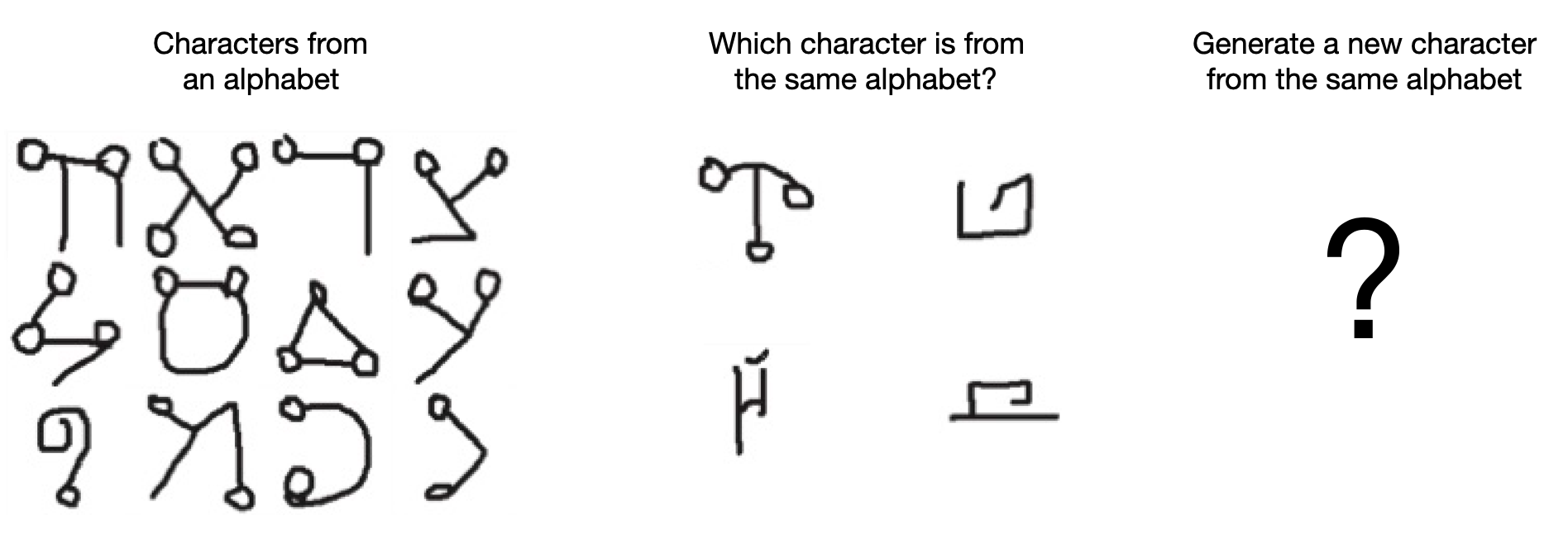
Or if I were to show you handwritten characters from a foreign alphabet, you’d be able to extract the high level pattern of that alphabet and recognize whether a new character is from that alphabet or even produce a new character from that alphabet.
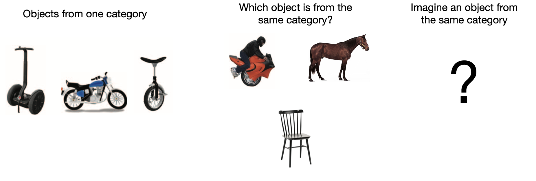
Another example is in categorizing new objects. I can show you a bike, a segway and a motorbike as examples of objects in a category and you’d instantly be able to classify a one-wheel motorbike as being in the same category despite not being either one of bike, segway or motorbike.
Sometimes, getting this more abstract knowledge out comes before the more specific knowledge and we can use this abstract knowledge to usefully guide our reasoning and decision making.
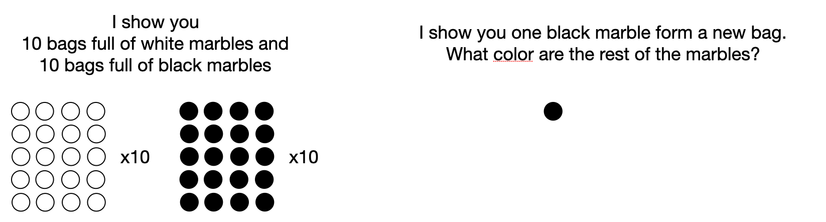
One of the main ways to model this is using hierarchical Bayesian models. Let’s illustrate this using a simple example from Kemp and colleagues. Say I show you a bunch of marble bags of either black or white marbles. The first ten bags I show you have 20 white marbles and 0 black marbles. The next ten bags I show you have 0 white marbles and 20 black marbles. Then the next bag I show you one marble and it’s black—what color do you think are the other marbles in this bag? Likely black because you inferred that the bags I give you have very extreme color proportions—either all white or all black. This is the sort of of abstract knowledge that can be inferred even before inferring the specifics about each individual bag.
I want to focus on the following questions
- Can we amortize inference in hierarchical models? This is required because inferences about this abstract knowledge should be quick.
- Can we learn such a hierarchical model from data if the abstract knowledge has a distributed representation—like an embedding vector? This is important as we scale these models to more complex data like utterances, handwritten characters or objects where it is harder to come up with an accurate, interpretable latent variable corresponding to the abstract knowledge.
Amortized inference
We’ll work with the marbles model from Kemp and colleagues which goes as follows
\(\alpha \sim \mathrm{Exponential}(1)\)
\(\beta \sim \mathrm{Dirichlet}([1, \dotsc, 1])\)
\(\theta_n \sim \mathrm{Dirichlet}(\alpha\beta)\)
\(x_n \sim \mathrm{Multinomial}(\theta_n)\)
The graphical model looks as follows
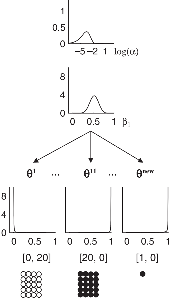
Our goal here is to train a neural net that gives us a posterior distribution over the the abstract \((\alpha, \beta)\) variables. As Kemp and colleagues explain, “when \(\alpha\) is small, the marbles in each individual bag are near-uniform in color (\(\theta_1\) is close to 0 or close to 1), and \(\beta\) determines the relative proportions of bags that are mostly black and bags that are mostly white. When \(\alpha\) is large, the color distribution for any individual bag is expected to be close to the color distribution across the entire population of bags (\(\theta_1\) is close to \(\beta_1\)).”
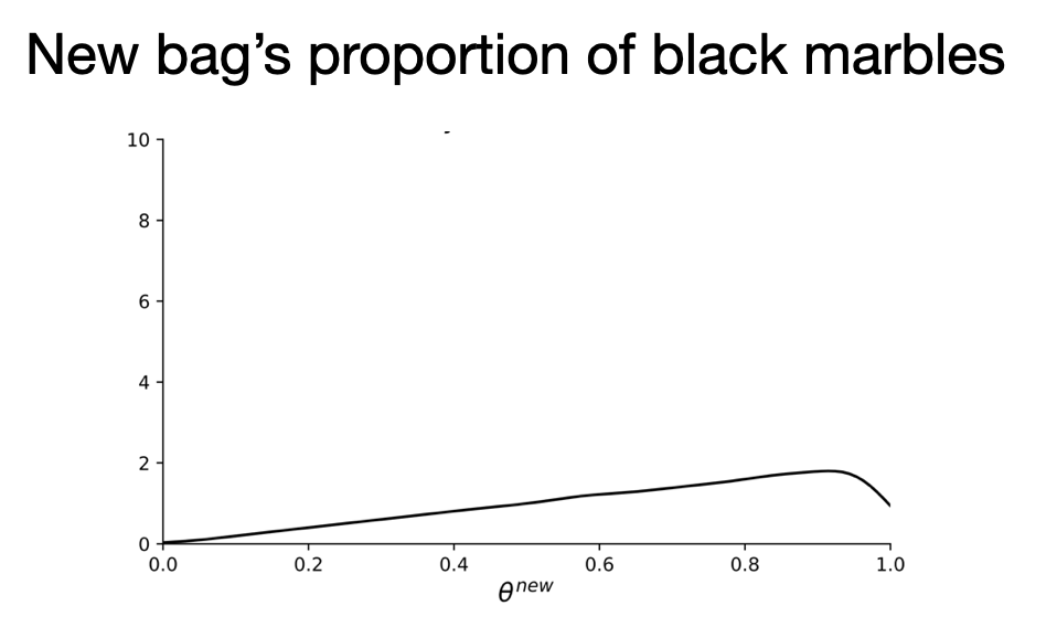
If we did MCMC inference, we’d predict high probability that \(\theta_{new}\) is skewed towards the right. That is, the new bag likely contains a lot of black marbles, based on the fact that the new bag has one black marble and the previous bags had extreme proportions–which is reflected through the \((\alpha, \beta)\) variables.
To amortize inference, we have to choose a factorization and the objective. Since the model is fixed, we can just use the wake-sleep or inference compilation objective and train the inference network on synthetic data generated from the fixed generative model.
Inference network factorizations
There are two natural choices for the factorization of the inference network: top-down and bottom-up as illustrated below
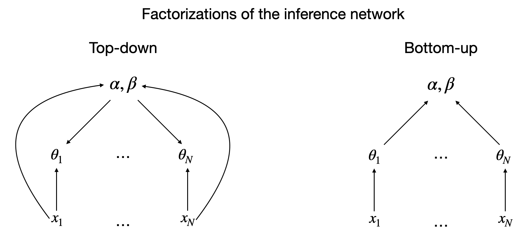
The top down factorization tells us that we infer the abstract knowledge first before inferring the more specific knowledge. This makes sense and mathematically respects the conditional independencies in the posterior but one could argue that it is hard to go directly from raw data to an abstract representation.
However, if our local variables were handwritten character parses, the bottom up factorization might be more suitable. It feels easier to infer the abstract variable from a bunch of parses rather than directly from a bunch of pixel images. However, this factorization doesn’t respect the conditional independencies in the posterior, unless we put in dependencies among the local variables. If we were to infer the proportion of marbles purely based on the current bag, ignoring the other bags, we wouldn’t be able to say that the newest bag is definitely full of black marbles. But knowing that the other bags have very extreme marble proportions would give us this information.
Results
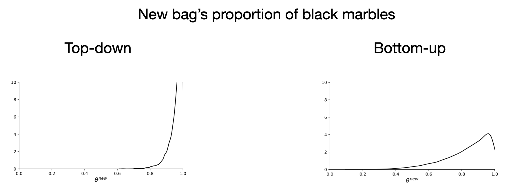
Take our favourite example. The top down factorization correctly infers that the new bag has a very high proportion of black marbles while the bottom up factorization is more unsure.
On the other hand, when the posterior on local variables isn’t conditionally dependent, the bottom up factorization does fine. For instance, if all the bags have 20 marbles, this already gives a lot of information about the local variables in a way that makes the abstract variable redundant. We can easily say that that the new bag has a high proportion of whites if we see 20 white marbles and don’t need information from the other bags.
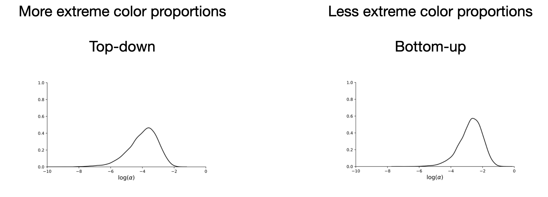
What about the abstract variable? Because the posterior on the local variables is inaccurate, it could also affect the posterior for the abstract variable. In the top down factorization, we should correctly infer the abstract variable. In the bottom up factorization, however, we infer that the bags have less extreme color proportions.
If we were to categorize new bags or if we were asked to generate new bags based on a set of bags, the bottom-up factorization is slightly worse. Conditioning on 10 all-black and 10 all-white bags
- a top-down factorization generates the following bags: (20, 0), (20, 0), (0, 20), (0, 20), (20, 0), (0, 20), (20, 0), (0, 20), (20, 0), (0, 20) while
- a bottom-up factorization generates (20, 0), (1, 19), (4, 16), (20, 0), (20, 0), (20, 0), (20, 0), (20, 0), (1, 19), (0, 20).
Answer to the first question
The answer to the first question above is: yes and the top-down factorization is preferable when the conditional dependency is needed.
Learning an abstract embedding vector
Of course, it’s not always possible to write such a nice generative model. Would it be possible to write a model in which the abstract latent variable has a distributed representation, that it is just an embedding vector? This would be a more generalizable strategy for modeling the more complex domains mentioned above.
For now we stay in the marbles domain and consider the following model family:
\(z \sim \mathrm{Normal}(0, I)\)
\(\theta_n \sim \mathrm{Dirichlet}(f_\psi(z))\)
\(x_n \sim \mathrm{Multinomial}(\theta_n)\)
where \(f_\psi\) is a 3-layer perceptron with ReLU non-linearities parameterized by \(\psi\) whose output is exponentiated and added to one. We use a top down factorization as it seems to be preferrable. Just instead of mapping to a distribution over \((\alpha, \beta)\), we map to a distribution on \(z\). We pick \(z\) to be two-dimensional so that it’s easy to visualize. We generate an infinite stream of datasets \(x_{1:N}\) and use the evidence lower bound (ELBO) objective to learn both the generative model and the inference network.
Example inference
Let’s have a look at our inferences. If we condition on bags with many marbles, the posteriors look OK.
However, if we only observe one black marble after observing 10 bags of all-white marbles and 10 bags of all-black marbles, we don’t get a peak on the high proportion of black marbles at all.
Learned generative model
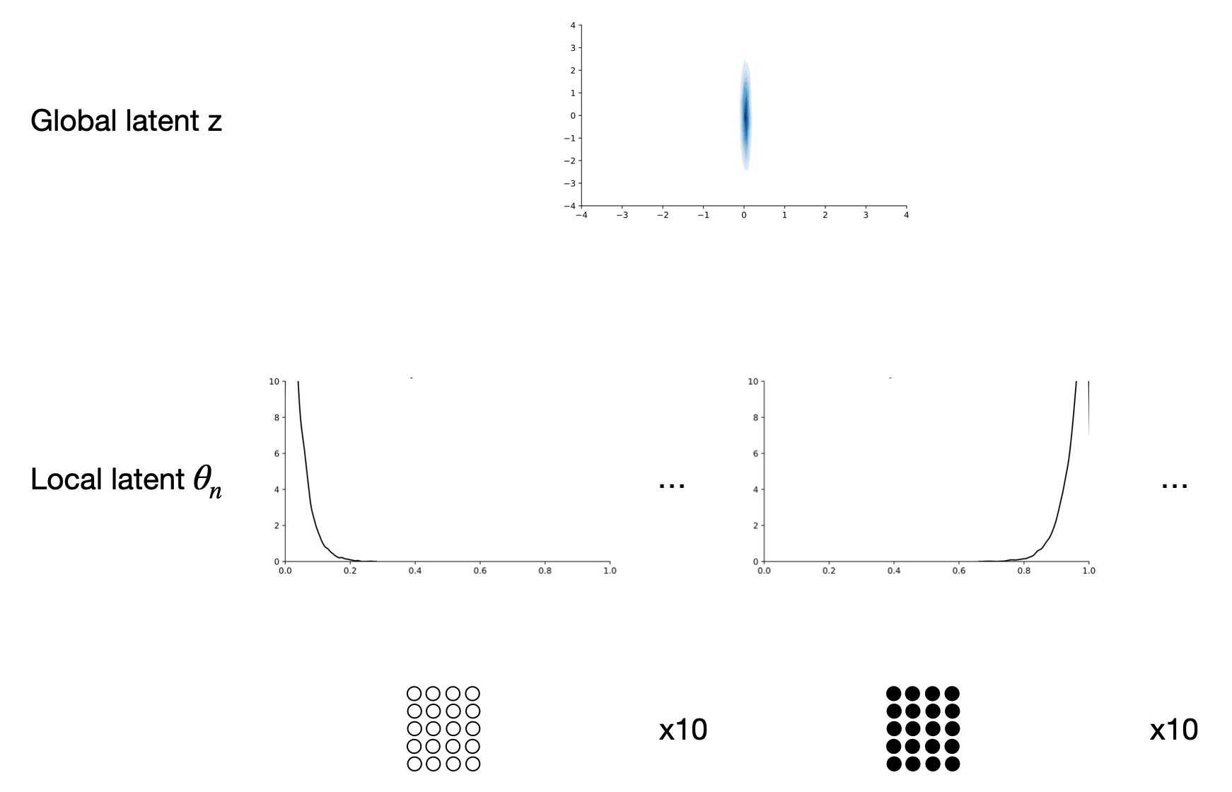
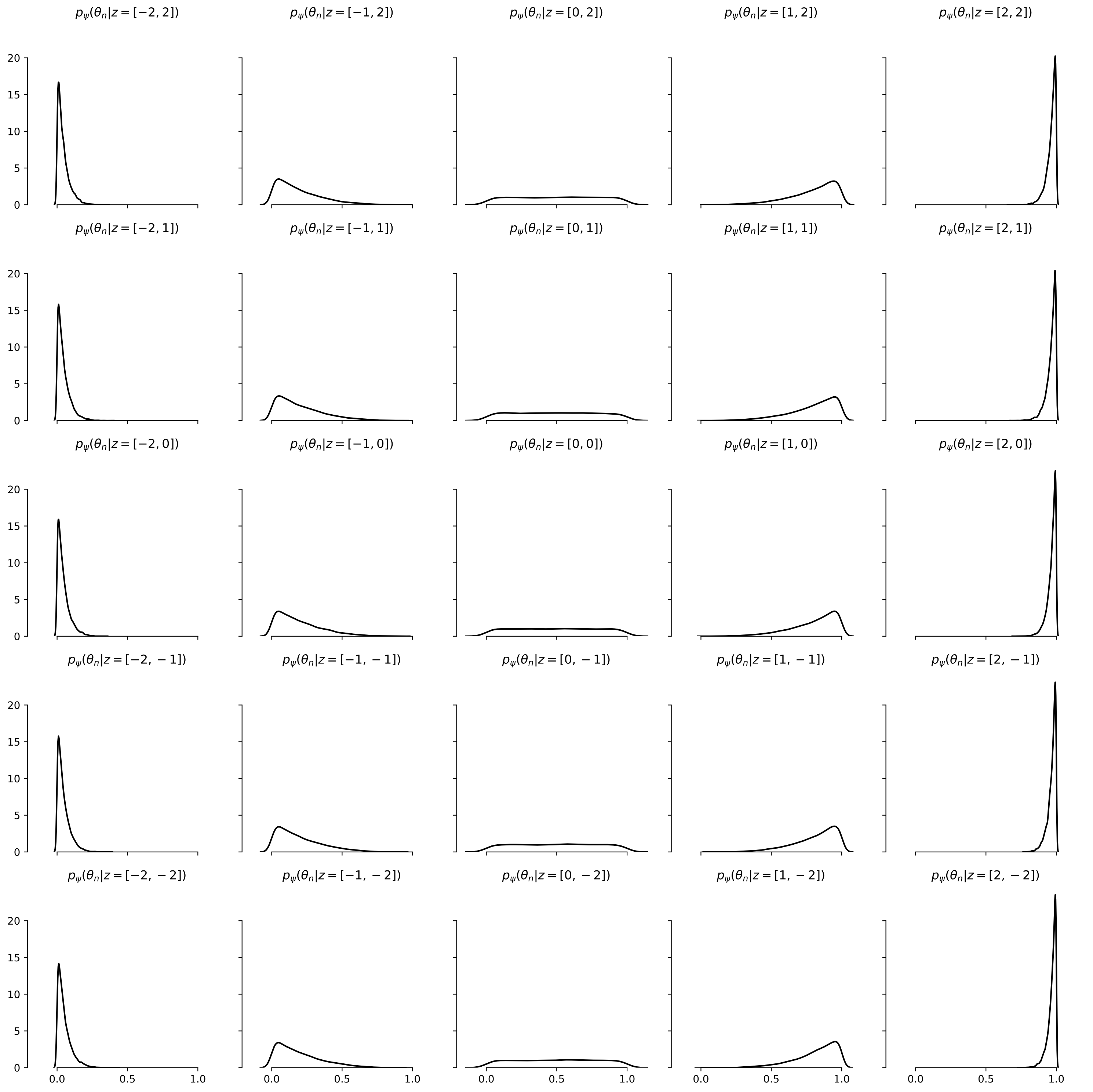
Let’s look at the learned generative model. The only learnable parameters are the weights \(\psi\) of the neural network \(f_\psi\) which is used within the conditional prior \(p_\psi(\theta_n \given z)\). Below, we show the conditional priors \(p_\psi(\theta_n \given z)\) for different \(z\)s. The first dimension affects both the peakiness and location of the distribution while the second element of \(z\) seems to be ignored.
Learned inference network
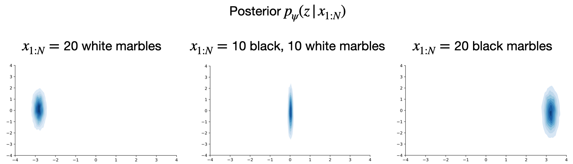
Now, let’s look at the learned inference network, conditioning on different marble bags \(x_{1:N}\).
- If we condition on bags with only white marbles, the posterior concentrates on the left region of the \(z\) space. Given our prior above, it is reasonable to expect that if we ask the model to generate new bags, it will generate bags with mostly white marbles: ((20, 0), (20, 0), (20, 0), (19, 1), (20, 0), (20, 0), (19, 1), (19, 1), (20, 0), (20, 0)).
- If we condition on bags with only black marbles, we get the opposite behavior: ((0, 20), (0, 20), (1, 19), (0, 20), (1, 19), (1, 19), (1, 19), (0, 20), (0, 20), (0, 20)).
- However, if we condition on 10 bags with all white marbles and 10 bags with all black marbles, our posterior is somewhere in the middle of the \(z\) space which corresponds to a uniform prior on \(\theta_n\) instead of a bimodal distribution (with one mode near 0 and the other near 1). Therefore, newly generated bags don’t have extreme marble color proportions: ((5, 15), (1, 19), (14, 6), (1, 19), (18, 2), (6, 14), (2, 18), (6, 14), (17, 3), (9, 11)).
Answer to the second question
We haven’t managed to fully answer the question above.
We have definitely learned a meaningful partitioning of the distributed latent variable \(z\):
- the left part corresponds to “bags with mostly white marbles”, and
- the right part corresponds to “bags with mostly black marbles”.
However, since our inference network is unimodal, we cannot capture concepts such as “bags with extreme color proportions” (mostly white OR mostly black) because this requires putting mass on both left and right parts of the latent space. Our model places mass in the middle instead which unfortunately captures the concept of “bags with completely random color proportions”.
There are two obvious potential solutions to this, neither of which seem to work so far:
- Use a higher dimensional latent space so that there can be single modes that capture more complex concepts like “bags with extreme color proportions”.
- Use a more expressive inference network in order to capture more modes.
[back]