Deep Q Network, Policy Gradients, Advantage Actor Critic

13 January 2018

This note draws from:

• https://keon.io/deep-q-learning/
• http://karpathy.github.io/2016/05/31/rl/
• https://www.alexirpan.com/rl-derivations/

Markov Decision Process (MDP)

An MDP with states \(S_{0:\infty}\) and actions \(A_{0:\infty}\) is specified by

• an initial density \(p(s_0)\),
• a transition density \(p(s_t \given s_{t - 1}), (t > 0)\), and
• a policy \(\pi(s_t \given a_t), (t \geq 0)\).

Denote the reward at time \(t\), \((t \geq 0)\), by \(r_t = R(s_t, a_t)\), where \(R\) is a reward function.

The MDP trace density is \begin{align} p(s_{0:\infty}, a_{0:\infty}) &= p(s_0) \pi(a_0 \given s_0) \prod_{t = 1}^\infty \left( p(s_t \given s_{t - 1}, a_{t - 1}) \pi(a_t \given s_t) \right). \end{align}

Deep Q Network (DQN)

There is a proof of convergence of the \(Q\)-learning algorithm for discrete spaces here. Forget about that in the deep reinforcement learning setting.

A \(Q\) function defined as \begin{align} Q(s_t, a_t) &= \E[r_t + \gamma r_{t + 1} + \cdots \given S_t = s_t, A_t = a_t] \\
&= \int (r_t + \gamma r_{t + 1} + \cdots) p(s_{t + 1} \given s_t, a_t) \prod_{\tau = t + 1}^\infty \left( \pi(a_\tau \given s_\tau) \cdot p(s_{\tau + 1} \given s_\tau, a_\tau) \right) \,\mathrm ds_{t + 1:\infty} \,\mathrm a_{t + 1:\infty} \\
&= r_t + \gamma \int (r_{t + 1} + \gamma r_{t + 2} + \cdots) p(s_{t + 1} \given s_t, a_t) \prod_{\tau = t + 1}^\infty \left( \pi(a_\tau \given s_\tau) \cdot p(s_{\tau + 1} \given s_\tau, a_\tau) \right) \,\mathrm ds_{t + 1:\infty} \,\mathrm a_{t + 1:\infty}. \label{eq:dqn-q} \end{align}

Now, note that for \((s_{t + 1}, a_{t + 1})\), the \(Q\) function is \begin{align} Q(s_{t + 1}, a_{t + 1}) &= \int (r_{t + 1} + \gamma r_{t + 2} + \cdots) p(s_{t + 2} \given s_{t + 1}, a_{t + 1}) \prod_{\tau = t + 2}^\infty \left( \pi(a_\tau \given s_\tau) \cdot p(s_{\tau + 1} \given s_\tau, a_\tau) \right) \,\mathrm ds_{t + 2:\infty} \,\mathrm a_{t + 2:\infty}. \end{align}

We use this in \eqref{eq:dqn-q} to obtain: \begin{align} Q(s_t, a_t) &= r_t + \gamma \int Q(s_{t + 1}, a_{t + 1}) p(s_{t + 1} \given s_t, a_t) \pi(a_{t + 1} \given s_{t + 1}) \,\mathrm ds_{t + 1} \,\mathrm da_{t + 1}. \label{eq:dqn-q-2} \end{align}

At the optimal policy, \begin{align} \pi^\ast(a \given s) = \delta_{\argmax_{a’} Q(s, a’)}(a), \end{align} where \(\delta_z\) is a delta mass at \(z\). Hence, at the optimal policy, we can write \eqref{eq:dqn-q-2} as follows: \begin{align} Q(s_t, a_t) &= r_t + \gamma \int \max_a Q(s_{t + 1}, a) p(s_{t + 1} \given s_t, a_t) \,\mathrm ds_{t + 1} \\
&= r_t + \gamma \E_{p(s_{t + 1} \given s_t, a_t)}[\max_a Q(s_{t + 1}, a)]. \end{align}

Hence, for random variables \((S_t, A_t, R(S_t, A_t), S_{t + 1})\) sampled from the MDP trace density, we would like the value of \begin{align} L_Q(S_t, A_t, R(S_t, A_t), S_{t + 1}) &= \left(Q(S_t, A_t) - (R(S_t, A_t) + \gamma \cdot \max_a Q(S_{t + 1}, a))\right)^2 \end{align} to be as small as possible.

In DQN, the \(Q\)-network \(Q_{\theta}\) is parameterized by \(\theta\). Given a sample \((s_t, a_t, r_t, s_{t + 1})\) from the marginal trace distribution \(p(s_{0:\infty}, a_{0:\infty})\), we can perform a stochastic gradient descent step to minimize \(\E[L_{Q_\theta}(S_t, A_t, R(S_t, A_t), S_{t + 1})]\) using the gradient \(\nabla_{\theta} L_{Q_\theta}(s_t, a_t, r_t, s_{t + 1})\).

Algorithm

• Initialize \(Q\)-network parameters \(\theta\).
• For some number of episodes:
  • Sample a trace \((s_0, a_0, r_0, \dotsc, s_T, a_T, r_T)\).
  • Record all tuples \((s_t, a_t, r_t, s_{t + 1})\) in a memory.
  • Sample a tuple \((s_t, a_t, r_t, s_{t + 1})\) from memory and perform a gradient update on \(\theta\) using \(\nabla_{\theta} L_{Q_\theta}(s_t, a_t, r_t, s_{t + 1})\).

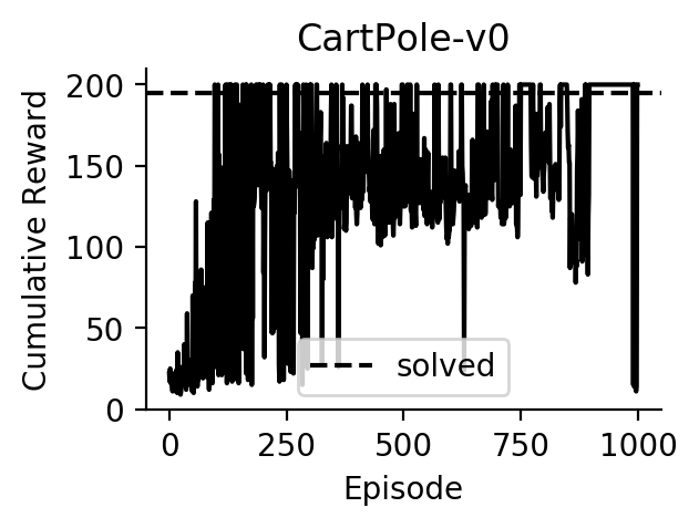
Experiments

Performance of DQN on CartPole:

Policy Gradients (PG)

In policy gradients, we parameterize the policy \(\pi_{\theta}(a \given s)\) by parameters \(\theta\). There is a policy network which typically maps from a state to the parameters of a distribution over actions.

We maximize the expected discounted rewards with respect to \(\theta\) directly using stochastic gradient ascent. The gradient can be rewritten as \begin{align} \nabla_\theta \E\left[ \sum_{t = 0}^T \gamma^t r_t \right] &= \nabla_\theta \int \left(\sum_{t = 0}^T \gamma^t r_t\right) p(s_{0:T}, a_{0:T}) \,\mathrm ds_{0:T} \,\mathrm da_{0:T} \\
&= \int \left(\sum_{t = 0}^T \gamma^t r_t\right) \left( p(s_0) \prod_{t = 1}^T p(s_t \given s_{t - 1}, a_{t - 1}) \right) \left( \nabla_\theta \prod_{t = 0}^T \pi_\theta(a_t \given s_t) \right) \,\mathrm ds_{0:T} \,\mathrm da_{0:T} \\
&= \int \left(\sum_{t = 0}^T \gamma^t r_t\right) \left( \nabla_\theta \sum_{t = 0}^T \log \pi_\theta(a_t \given s_t) \right) p(s_{0:T}, a_{0:T}) \,\mathrm ds_{0:T} \,\mathrm da_{0:T} \\
&= \E\left[ \left(\sum_{t = 0}^T \gamma^t r_t\right) \left( \nabla_\theta \sum_{t = 0}^T \log \pi_\theta(a_t \given s_t) \right) \right]. \label{eq:pg} \end{align}

Hence, we can get an unbiased estimate of the gradient by sampling \((s_0, a_0, \dotsc, s_T, a_T) \sim p(s_{0:T}, a_{0:T})\) and evaluating \(\left(\sum_{t = 0}^T \gamma^t r_t\right) \nabla_\theta\left( \sum_{\tau = 0}^T \log \pi_\theta(a_\tau \given s_\tau) \right)\).

Algorithm

• Initialize policy network parameters \(\theta\).
• For some number of episodes:
  • Sample a trace \((s_0, a_0, r_0, \dotsc, s_T, a_T, r_T)\).
  • Perform a gradient update on \(\theta\) using \(\left(\sum_{t = 0}^T \gamma^t r_t\right) \left( \nabla_\theta \sum_{t = 0}^T \log \pi_\theta(a_t \given s_t) \right)\).

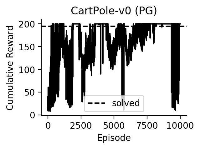
Experiments

Performance of Policy Gradients on CartPole:

Advantage Actor Critic (A2C)

We are going to use the following fact: \begin{align} \E[\nabla_\theta \log \pi_\theta (a_t \given s_t)] &= \int \nabla_\theta \log \pi_\theta(a_t \given s_t) \pi_\theta(a_t \given s_t) \,\mathrm da_t \\
&= \int \nabla_\theta \pi_\theta(a_t \given s_t) \,\mathrm da_t \\
&= \nabla_\theta \int \pi_\theta(a_t \given s_t) \,\mathrm a_t \\
&= \nabla_\theta 1 \\
&= 0. \label{eq:a2c-zero-grad} \end{align}

Starting from \eqref{eq:pg}, we have: \begin{align} \nabla_\theta \E\left[ \sum_{t = 0}^T \gamma^t r_t \right] &= \E\left[ \left(\sum_{t = 0}^T \gamma^t r_t\right) \left( \nabla_\theta \sum_{t = 0}^T \log \pi_\theta(a_t \given s_t) \right) \right] \\
&= \sum_{t = 0}^T \E\left[ \left(\sum_{\tau = 0}^T \gamma^\tau r_\tau\right) \nabla_\theta \log \pi_\theta(a_t \given s_t) \right] \\
&= \sum_{t = 0}^T \left( \E\left[ \left(\sum_{\tau = 0}^{t - 1} \gamma^\tau r_\tau\right) \nabla_\theta \log \pi_\theta(a_t \given s_t) \right] + \E\left[ \left(\sum_{\tau = t}^T \gamma^\tau r_\tau\right) \nabla_\theta \log \pi_\theta(a_t \given s_t) \right]\right) \\
&= \sum_{t = 0}^T \left( \E_{p(s_{0:t - 1}, a_{0:t - 1}) p(s_t \given s_{t - 1}, a_{t - 1})}\left[\left(\sum_{\tau = 0}^{t - 1} \gamma^\tau r_\tau\right) \E_{\pi_\theta(a_t \given s_t)}\left[\nabla_\theta \log \pi_\theta(a_t \given s_t)\right]\right] + \E\left[ \left(\sum_{\tau = t}^T \gamma^\tau r_\tau\right) \nabla_\theta \log \pi_\theta(a_t \given s_t) \right]\right) \\
&= \sum_{t = 0}^T \E\left[ \left(\sum_{\tau = t}^T \gamma^\tau r_\tau\right) \nabla_\theta \log \pi_\theta(a_t \given s_t) \right] && \text{(use \eqref{eq:a2c-zero-grad})} \\
&= \sum_{t = 0}^T \E\left[ \left(\left(\sum_{\tau = t}^T \gamma^\tau r_\tau\right) - b(s_t)\right) \nabla_\theta \log \pi_\theta(a_t \given s_t) \right] && \text{(use \eqref{eq:a2c-zero-grad})}, \label{eq:a2c} \end{align} where \(b(s_t)\) is called a baseline. The more \(b(s_t)\) is correlated with \(\left(\sum_{\tau = t}^T \gamma^\tau r_\tau\right)\), the lower the variance of the gradient estimator.

Approximation of the Value Function

In A2C, \(b(s_t)\) is usually set to an approximation to the value function \(V(s_t)\) which is defined as \begin{align} V(s_t) &= \E[r_t + \gamma r_{t + 1} + \cdots \given S_t = s_t]. \end{align}

Let \(V(s_t)\) be a function parameterized by \(\phi\). Then, using the \(n\)-step relationship for value function (eq. 14 in here), it can be optimized by minimizing the following loss with respect to \(\phi\): \begin{align} L_V(s_t, r_t, \dotsc, s_{t + n - 1}, r_{t + n - 1}, s_{t + n}) = \left( \left(\sum_{k = 0}^{n - 1} \gamma^k r_{t + k}\right) + \gamma^n V^-(s_{t + n}) - V(s_t) \right)^2, \label{eq:loss-v} \end{align} where the minus superscript denotes detaching \(\phi\) from the computation graph. This is optimized in parallel with the optimization of the policy parameters \(\theta\).

\(n\)-step A2C

Starting from \eqref{eq:a2c}, we derive the \(n\)-step A2C update as described in Algorithm S3 of the original A3C paper:

\begin{align} &\sum_{t = 0}^T \E\left[ \left(\left(\sum_{\tau = t}^T \gamma^\tau r_\tau\right) - V(s_t)\right) \nabla_\theta \log \pi_\theta(a_t \given s_t) \right] \\
&\approx \sum_{\color{red}{i = 0}}^{\color{red}{n - 1}} \E\left[ \left(\left(\sum_{\tau = \color{red}{i}}^T \gamma^\tau r_\tau \right) - V(s_{\color{red}{i}})\right) \nabla_\theta \log \pi_\theta(a_{\color{red}{i}} \given s_{\color{red}{i}}) \right] && \text{(sum to } (n - 1) \text{ instead of } T \text{)} \\
&\approx \sum_{i = 0}^{n - 1} \E\left[\left(\left(\sum_{\tau = \color{red}{t + i}}^T \gamma^\tau r_\tau\right) - V(s_{\color{red}{t + i}})\right) \nabla_\theta \log \pi_\theta(a_{\color{red}{t + i}} \given s_{\color{red}{t + i}})\right] && \text{(sum from } t \text{ instead of } 0 \text{)} \\
&\approx \sum_{i = 0}^{n - 1} \E\left[\left(\left(\sum_{\tau = t + i}^T \gamma^{\tau \color{red}{- (t + i)}} r_\tau\right) - V(s_{t + i})\right) \nabla_\theta \log \pi_\theta(a_{t + i} \given s_{t + i})\right] && \text{(start discounting from } 0 \text{ instead of } (t + i) \text{)}\\
&\approx \sum_{i = 0}^{n - 1} \E\left[\left(\left(\sum_{\tau = t + i}^{\color{red}{t + n - 1}} \gamma^{\tau - (t + i)} r_\tau\right) \color{red}{+ \gamma^{n - i} V(s_{t + n})} - V(s_{t + i})\right) \nabla_\theta \log \pi_\theta(a_{t + i} \given s_{t + i})\right] && \text{(approximate tail of the inner sum by the value function)} \\
&\approx \sum_{i = 0}^{n - 1} \E\left[\left(\left(\sum_{\color{red}{j = 0}}^{\color{red}{n - i - 1}} \gamma^{\color{red}{j}} r_{\color{red}{t + i + j}}\right) + \gamma^{n - i} V(s_{t + n}) - V(s_{t + i})\right) \nabla_\theta \log \pi_\theta(a_{t + i} \given s_{t + i})\right] && \text{(change inner index from } \tau \text{ to } j \text{)}. \label{eq:n-step-a2c} \end{align}

Noting the similar form of \eqref{eq:loss-v} and \eqref{eq:n-step-a2c}, we define the so-called advantage function, parameterized by \(\phi\): \begin{align} A(s_{t + i}, r_{t + i}, \dotsc, s_{t + n - 1}, r_{t + n - 1}, s_{t + n}) &= \left(\sum_{j = 0}^{n - i - 1} \gamma^{j} r_{t + i + j}\right) + \gamma^{n - i} V^-(s_{t + n}) - V(s_{t + i}). \end{align} Hence, given \((s_t, r_t, \dotsc, s_{t + n - 1}, r_{t + n - 1}, s_{t + n})\), the policy and value-function losses are: \begin{align} L_\pi(s_t, r_t, \dotsc, s_{t + n - 1}, r_{t + n - 1}, s_{t + n}) &= -\sum_{i = 0}^{n - 1} A(s_{t + i}, r_{t + i}, \dotsc, s_{t + n - 1}, r_{t + n - 1}, s_{t + n})^- \log \pi_\theta(a_{t + i} \given s_{t + i}) \\
L_V(s_t, r_t, \dotsc, s_{t + n - 1}, r_{t + n - 1}, s_{t + n}) &= \sum_{i = 0}^{n - 1} A(s_{t + i}, r_{t + i}, \dotsc, s_{t + n - 1}, r_{t + n - 1}, s_{t + n})^2. \end{align}

Implementations:

• A3C paper pseudocode
• Pytorch implementation
• Another Pytorch implementation
• Tensorflow implementation

Algorithm

• Initialize policy network parameters \(\theta\) and value network parameters \(\phi\)
• For some number of episodes:
  • Sample a trace \((s_t, r_t, \dotsc, s_{t + n - 1}, r_{t + n - 1}, s_{t + n})\).
  • Perform a gradient update on \(\theta\) using \(\nabla_\theta L_\pi(s_t, r_t, \dotsc, s_{t + n - 1}, r_{t + n - 1}, s_{t + n})\).
  • Perform a gradient update on \(\phi\) using \(\nabla_\phi L_V(s_t, r_t, \dotsc, s_{t + n - 1}, r_{t + n - 1}, s_{t + n})\).

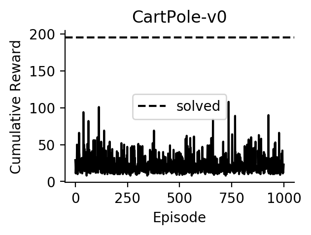
Experiments

Performance of A2C on CartPole (doesn’t work yet; TODO: make it work):

[back]